GaussianCross: Cross-modal Self-supervised 3D Representation Learning via Gaussian Splatting

TL;DR

GaussianCross converts scale-inconsistent point clouds into a unified cuboid-normalized Gaussian representation, then distils appearance, geometry and semantics into a 3D feature field — self-supervised pre-training with no labels and no model collapse.

Abstract

The significance of informative and robust point representations has been widely acknowledged for 3D scene understanding. Despite existing self-supervised pre-training counterparts demonstrating promising performance, the model collapse and structural information deficiency remain prevalent due to insufficient point discrimination difficulty, yielding unreliable expressions and suboptimal performance.

In this paper, we present GaussianCross, a novel cross-modal self-supervised 3D representation learning architecture integrating feed-forward 3D Gaussian Splatting (3DGS) techniques. GaussianCross seamlessly converts scale-inconsistent 3D point clouds into a unified cuboid-normalized Gaussian representation without missing details, enabling stable and generalizable pre-training. A tri-attribute adaptive distillation splatting module then constructs a 3D feature field, capturing appearance, geometry and semantic cues synergetically to maintain cross-modal consistency.

We evaluate on ScanNet, ScanNet200 and S3DIS. GaussianCross shows prominent parameter and data efficiency, and strong generalization, improving full fine-tuning accuracy by 9.3% mIoU and 6.1% AP₅₀ on ScanNet200 semantic and instance segmentation.

Contributions

01 Cross-modal self-supervised learning with generalizable Gaussian Splatting
A pre-training architecture for 3D scene understanding that learns directly from raw scans, with none of the per-scene optimization vanilla 3DGS depends on.
02 Cuboid-normalized Gaussian initialization
Scenes become structured 3D Gaussians inside one shared cuboid domain, absorbing the scale inconsistency between scans without discarding detail.
03 Tri-attribute adaptive distillation splatting
Appearance, geometry and semantics are captured jointly, distilling knowledge from a 2D visual foundation model into the 3D representation.
04 Consistent gains across scene understanding tasks
One set of pre-trained weights transfers to semantic and instance segmentation on ScanNet, ScanNet200 and S3DIS, ahead of previous state-of-the-art methods.

How it works

A raw scan goes in, half of it gets thrown away

The scene 𝐏_r is masked at γ = 50% and grid-subsampled to 𝐏_g, then encoded by a sparse 3D backbone ℰ_φ into per-point features 𝐅_s. Everything downstream exists only to supervise this encoder — after pre-training it is the single artefact we keep and transfer.

input𝐏_r = {𝐂_r, 𝐀_r}

mask ratioγ = 50%

output𝐅_s ∈ ℝ^m×d_s

Every scene is folded into the same cuboid

3D scans arrive at wildly different scales, which is exactly what breaks per-scene 3DGS. Coordinates are mapped into a unit cube by ℐ and discretized by 𝒱 into X×Y×Z voxels; sparse features are scattered into a dense volume 𝐅_v and refined by a 3D CNN ℰ_θ^den into 𝐅_d. Each voxel centre becomes a coarse Gaussian mean ν — no SfM, no per-scene optimization, no lost detail.

transformℐ ∘ 𝒱

anchors𝐂_v → ν

output𝐅_d ∈ ℝ^X×Y×Z×d_o

Voxels become Gaussians — and a semantic field

Every one of the X×Y×Z voxel centres is an anchor. MLP heads 𝒢 decode a position offset δ, quaternion q, scale s, colour c and opacity σ for each, plus a semantic embedding f that turns the primitive set into a queryable feature field. The refined mean is μ = ν + δ; anchors whose opacity falls below τ = 0.3 are pruned, which is what thins the full lattice down to a usable scene.

primitive{μ, q, s, c, σ, f}

pruneσ ≤ τ = 0.3

offsetδ = tanh(𝒢_δ)·Δ

Three renderings have to agree at once

The Gaussians are rasterized from M = 5 randomly sampled posed views into colour 𝒞, feature ℱ and depth 𝒟 maps. Colour and depth are matched to the real RGB-D frames with ℓ1 losses. The rendered feature map is low-dimensional, so a projection head 𝒫_ψ lifts it to ℱ before a cosine loss aligns it with ℱ* — the latent of that same real image under a frozen 2D foundation model 𝒳_f. Any such model will do; we use RADIOv2.5. Appearance, geometry and semantics must be consistent from every viewpoint — that joint constraint is what stops the representation from collapsing.

viewsM = 5, 480×640

2D priorfrozen 𝒳_f ❄

totalλ₁ℒ_img + λ₂ℒ_dep + λ₃ℒ_sem

Original architecture figure from the paper

GaussianCross pipeline figure from the paper. — **Fig. 2 of the paper.** The pipeline commences with cuboid-normalized Gaussian initialization to establish coarse primitive means. Gaussian properties are decoded by 𝒢 with a feature field, and tri-attribute adaptive distillation splatting enforces cross-modal consistency.

Results

Fig. 01 · ScanNet — what a single query point retrieves

LOADING…

drag to orbit · scroll to zoom

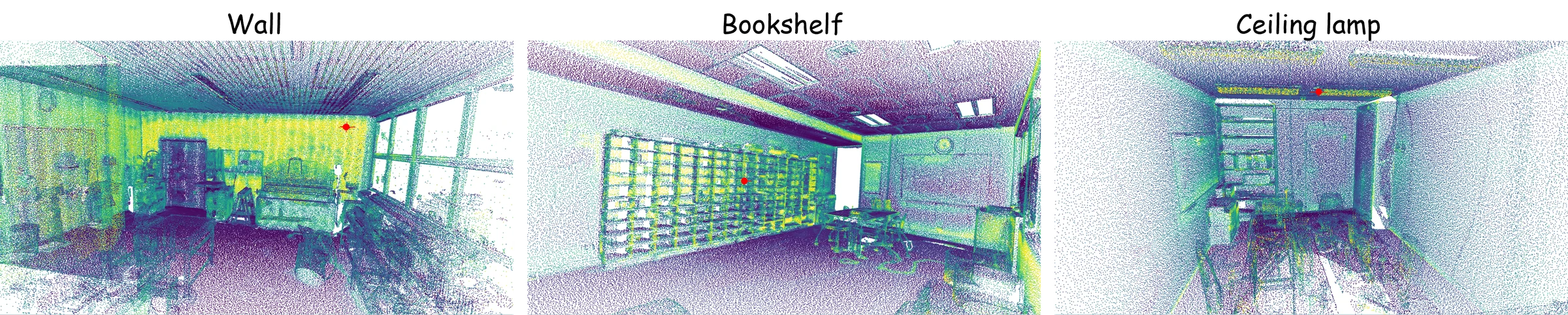
ScanNet. The encoder's features, then one query point (red cross), then every point coloured by its cosine similarity to that query — bright means alike. Query one armchair and the other armchairs light up; nothing here was ever labelled. These are the five scenes of Fig. 6 in the paper, with the same query points.

Cosine similarity heat maps on S3DIS. — **S3DIS.** Pre-training only ever saw ScanNet. The same query behaviour holds on a dataset the encoder has never seen, with no fine-tuning.

Cosine similarity heat maps on ScanNet++. — **ScanNet++.** Held-out scenes at a different capture quality — again with no fine-tuning and no labels.

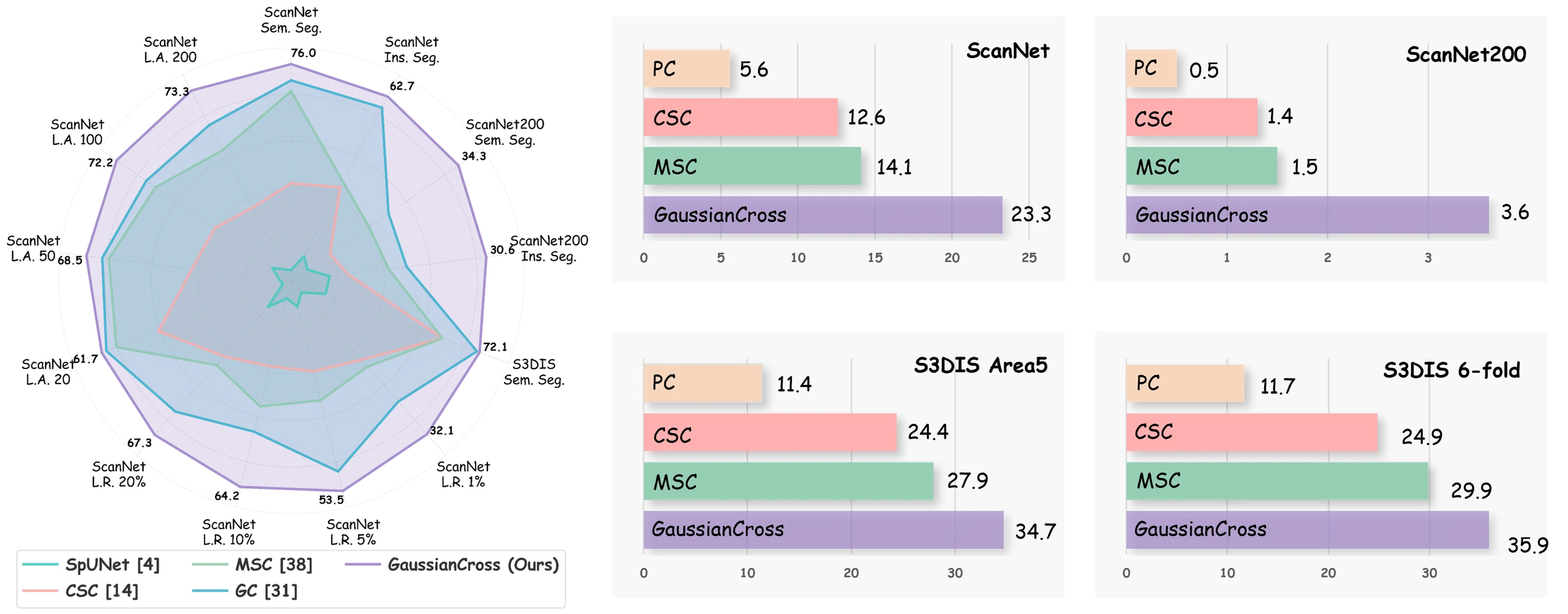
Radar chart and bar charts comparing GaussianCross against SpUNet, CSC, MSC and GC across ScanNet, ScanNet200 and S3DIS. — **Across the board.** Full fine-tuning (left) and linear probing (right) on semantic segmentation, instance segmentation and limited-data regimes.

trained from scratch self-supervised pre-training supervised pre-training underline = second best subscript = gain over the scratch baseline

Semantic segmentation, full fine-tuning

mIoU on the validation splits. Pre-training uses no labels of any kind.

Method				ScanNet	ScanNet200	S3DIS
	Venue	Pre-training data	Type	Val mIoU	Val mIoU	Area 5	6-fold
Supervised learning from scratch
PointNeXt	NeurIPS 2022	—	—	71.5	—	70.5	74.9
StFormer	CVPR 2022	—	—	74.3	—	72.0	—
PTv1	ICCV 2021	—	—	70.6	27.8	70.4	65.4
PTv2	NeurIPS 2022	—	—	75.4	30.2	71.6	75.1
SpUNet (baseline)	CVPR 2019	—	—	72.2	25.0	66.3	72.4
Self-supervised pre-training
GS³	arXiv 2024	ScanNet	Rendering	73.4+1.2	—	70.1+3.8	—
Ponder	CVPR 2023	ScanNet	Rendering	73.5+1.3	—	—	—
CSC	CVPR 2021	ScanNet	Contrast	73.8+1.6	26.4+1.4	70.7+4.4	75.5+3.1
PC	ECCV 2020	ScanNet	Contrast	74.1+1.9	26.2+1.2	70.3+4.0	74.7+2.3
MSC	CVPR 2023	ScanNet, ArkitScenes	Contrast	75.5+3.3	32.0+7.0	70.7+4.4	—
GC	CVPR 2024	ScanNet	Contrast	75.7+3.5	30.0+5.0	72.0+5.7	—
PPT Unsup.	CVPR 2024	ScanNet, Structure3D, S3DIS	Contrast	75.8+3.6	30.4+5.4	71.9+5.6	—
GaussianCross	MM 2025	ScanNet	Rendering	76.0+3.8	34.3+9.3	72.1+5.8	76.8+4.4
Supervised pre-training · uses labels, shown for reference
PPT Sup.	CVPR 2024	ScanNet, Structure3D, S3DIS	3D Sup.	76.4+4.2	31.9+6.9	72.7+6.4	78.1+5.7
PonderV2	arXiv 2024	ScanNet, Structure3D, S3DIS	2D Sup.	77.0+4.8	32.3+7.3	73.2+6.9	79.9+7.4
ARKit LM	CVPR 2025	ALS200, ScanNet/ScanNet200	3D Sup.	77.0+4.8	30.6+5.6	—	—

Instance segmentation

PointGroup decoder, full fine-tuning.

	ScanNet			ScanNet200
Method	AP₂₅	AP₅₀	mAP	AP₂₅	AP₅₀	mAP
PointGroup	72.8	56.9	36.0	32.2	24.5	15.8
PC	—	58.0	—	—	24.9	—
GS³	—	59.2	37.0	—	—	—
CSC	—	59.4	—	—	25.2	—
MSC	74.7	59.6	39.3	34.3	26.8	17.3
GC	—	62.3	—	—	27.5	—
GaussianCross	77.0+4.2	62.7+6.2	40.8+4.8	38.4+5.8	30.6+6.1	20.6+4.8

Linear probing

Backbone frozen, one linear layer trained (<0.1% of parameters).

	ScanNet		ScanNet200		S3DIS A5		S3DIS 6-fold
Method	mIoU	mAcc	mIoU	mAcc	mIoU	mAcc	mIoU	mAcc
SpUNet (full sup.)	72.2	80.2	25.0	32.9	66.3	72.5	72.4	80.9
PC	5.6	9.7	0.5	0.9	11.4	18.6	11.7	19.0
CSC	12.6	18.1	1.3	2.1	24.4	32.0	24.9	32.5
MSC	14.1	20.3	1.5	2.5	27.9	35.5	29.9	37.9
GaussianCross	23.3	30.9	3.6	5.3	34.7	44.1	35.9	45.5

Data efficiency on ScanNet

mIoU when only a fraction of scenes, or a handful of annotated points per scene, is available.

	Limited scenes (% of the training set)				Limited annotations (labelled points per scene)
Method	1%	5%	10%	20%	20	50	100	200
SpUNet (baseline)	26.0	47.8	56.7	62.9	41.9	53.9	62.2	65.5
CSC	28.9	49.8	59.4	64.6	55.5	60.5	65.9	68.2
MSC	29.2	50.7	61.0	64.9	60.1	66.8	69.7	70.7
GC	30.7	52.9	62.0	66.5	61.2	67.3	70.3	71.8
PPT	31.3	52.3	62.8	66.4	60.6	67.5	70.8	72.2
GaussianCross	32.1	53.5	64.2	67.3	61.7	68.5	72.2	73.3
Δ vs. baseline	+6.1	+5.7	+7.5	+4.4	+19.8	+14.6	+10.0	+7.8

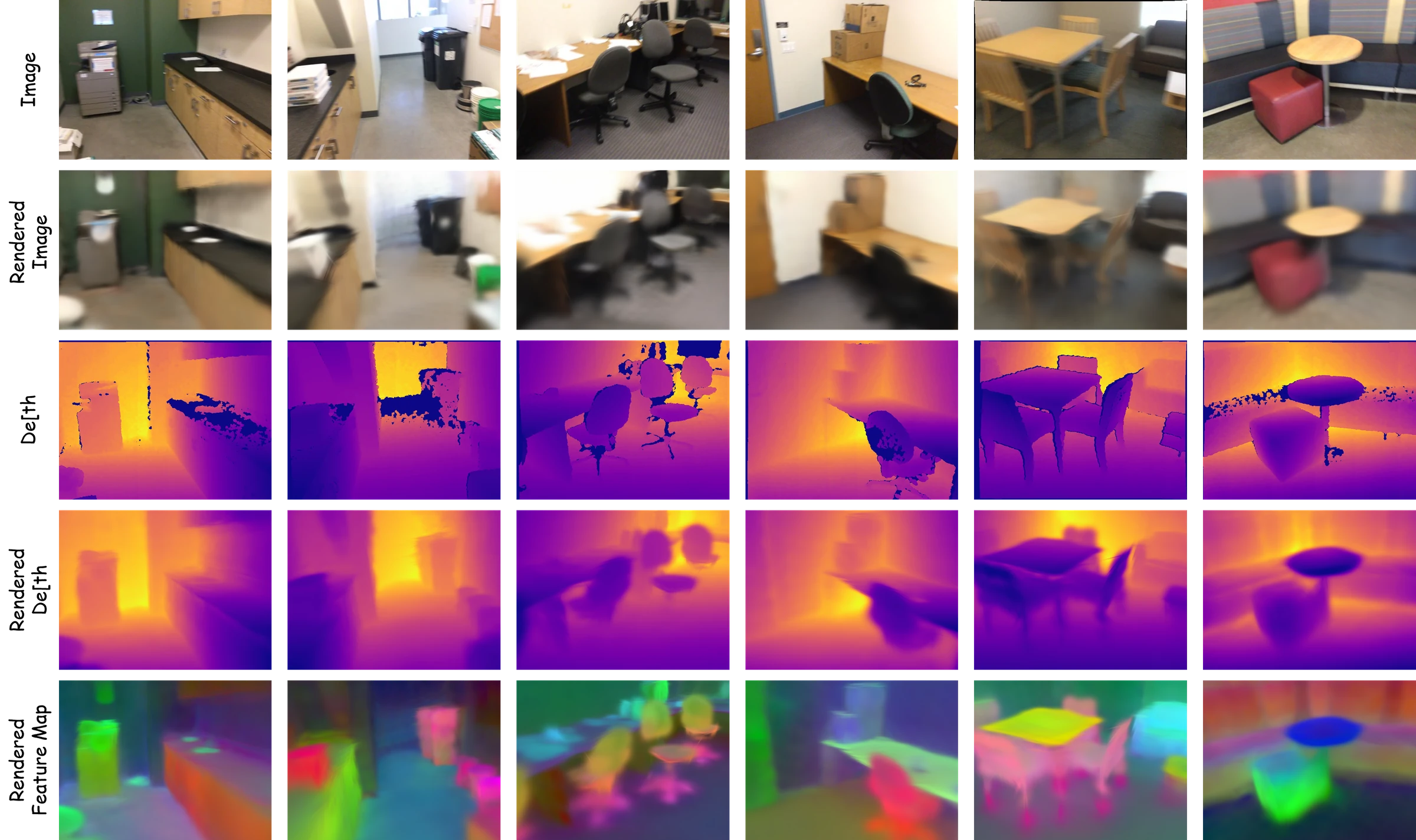
Tri-attribute rendering: appearance, geometry and semantics. — **Tri-attribute rendering.** Appearance, geometry and semantics rendered from the same Gaussian field.

GaussianCross

Abstract

How it works

A raw scan goes in, half of it gets thrown away

Every scene is folded into the same cuboid

Voxels become Gaussians — and a semantic field

Three renderings have to agree at once

Results

Semantic segmentation, full fine-tuning

Instance segmentation

Linear probing

Data efficiency on ScanNet

Citation